Time Series Analysis (Lecture 4 Part 2): Bounds Cointegration Test in EViews

After unit root testing, what next?

In the Part 1 of this structured tutorials, we discussed Scenario 1: when the series are stationary in levels that is I(0) series and Scenario 2: when they are stationary at first difference. In the first scenario, it implies that any shock to the system in the short run quickly adjusts to the long run. Hence, only the long run model should be estimated.  While for the second scenario, the relevance of the variables in the model is required, therefore there is need to test for cointegration. If there is cointegration, specify the long-run model and estimate VECM but if otherwise, specify only the short-run model and apply the VAR estimation technique and not VECM. In today’s lecture we consider the third scenario of when the variables are integrated of different orders.

Scenario 3: The series are integrated of different orders? 

1.    Should in case the series are integrated of different orders, like the second scenario, cointegration test is also required but the use of Johansen cointegration test is no longer valid.

2.    The appropriate cointegration test is the Bounds test for cointegration proposed by Pesaran, Shin and Smith (2001)

3. The estimation technique to apply is not VAR but the autoregressive distributed lag (ARDL) model.

4.  Similar to scenario 2, if series are not cointegrated based on Bounds test, we are expected to estimate only the short run. That is, run only the ARDL model (where variables are neither lagged nor differenced). It is the static form of the model. 

5.    However, both the long run and short run models are valid if there is cointegration. That is, run both ARDL and ECM models.

                                                                        

Bounds Cointegration Test in EViews

In this example, we use the Dar.xlsx data on Nigeria from 1981 to 2014 and the variables are the log of manufacturing value-added (lnmva), real exchange rate (rexch) and gross domestic growth rate (gdpgr). The model examines the effect of real exchange rate on manufacturing sector while controlling for economic growth.

Note: Cointegration test should be performed on the level form of the variables and not on their first difference. It is okay to also use the log-transformation of the raw variables, as I have done in this example.

Step 1: Load data into EViews (see video on how to do this)

Step 2: Open variables as a Group data (see video on how to do this) and save under a new name

Step 3: Go to Quick >> Estimate Equation >> and specify the static form of the model which is stated as: lnmva_t = b₀ + b₁rexch_t + b₂gdpgr_t + u_t in the Equation Estimation Window

EViews Estimation Equation Dialog Box
Source: CrunchEconometrix

Step 4: Choose the appropriate estimation technique

Click on the drop-down button in front of Method under Estimation settings and select ARDL – Auto regressive Distributed Lag Models

Source: CrunchEconometrix

Step 5: Choose the appropriate maximum lags and trend specification

The lag length must be selected such that the degrees of freedom (defined as n - k) must not be less than 30. The Constant option under the Trend specification is also selected.

EViews: Lags Option
Source: CrunchEconometrix

Step 6: Choose the appropriate lag selection criterion for optimal lag

Click on Options tab, then click on the drop-down button under Model Selection Criteria and select the Akaike info Criterion (AIC), then click Ok.

EViews: Information Criterion Selection
Source: CrunchEconometrix

Step 7: Estimate the model based on Steps 3 to 6

EViews: ARDL Output
Source: CrunchEconometerix

Step 8: Evaluate the preferred model and conduct Bounds test

The hypothesis is stated as:

H₀: no cointegrating equation

H₁: H₀ is not true

Rejection of the null hypothesis is at the relevant statistical level, 10%, 5% level, 1%.

a. Click on View on the Menu Bar

b. Click on Coefficient Diagnostics

c. Select the Bounds Test option

The following result is displayed below:

Here is the EViews result on the ARDL Bounds Test of lnmva, rexch and gdpgr:

EViews: ARDL Bounds Test Result
Source: CrunchEconometrix

Step 9: Interpret your result appropriately using the following decision criteria

The three options of the decision criteria are as follows:

1.    If the calculated F-statistic is greater than the critical value for the upper bound I(1), then we can conclude that there is cointegration that is there is long-run relationship.

2.    If the calculated F-statistic falls below the critical value for the lower bound I(0) bound, then we conclude that there is no cointegration, hence, no long-run relationship

3.    The test is considered inconclusive if the F-statistic falls between the lower bound I(0) and the upper bound I(1).

Decision: The obtained F-statistic of 0.6170 falls below the lower bound I(0), hence, we will consider only short run models since the variables show no evidence of a long-run relationship as indicated by the results from the Bounds test.

[Watch video on how to conduct Bounds test for cointegration in EViews]

If there are comments or areas requiring further clarification, kindly post them below….

Time Series Analysis (Lecture 4 Part 1): Johansen Cointegration Test in EViews

After unit root testing, what next?

The outcome of unit root testing matters for the empirical model to be estimated. The following scenarios explain the implications of unit root testing for further analysis.  Still drawing on the previous tutorials (see here for EViews, Stata and Excel) on unit root testing with the augmented Dickey-Fuller procedure (see videos), we are using the same data from Gujarati and Porter Table 21.1 quarterly data of 1970q1 to 1991q4. The variables in question are pce, pdi and gdp in natural logarithms.

Scenario 1:  When series under scrutiny are stationary in levels.

In this scenario, it is assumed that lnpce, lnpdi and lngdp are stationary in levels, that is, they are I(0) series (integrated of order zero).  In this situation, performing a cointegration test is not necessary. This is because any shock to the system in the short run quickly adjusts to the long-run. Consequently, only the long run model should be estimated using OLS (where variables are neither lagged nor differenced). It is the static form of the model. In essence, the estimation of short run model is not necessary if series are I(0).  

Scenario 2: When series are stationary in first differences.

1.    Under this scenario, the series are assumed to be non-stationary but became stationary after first difference

2.    One special feature of this is that they are of the same order of integration.

3. Under this scenario, the model in question is not entirely useless although the variables are unpredictable. To verify further the relevance of the model, there is need to test for cointegration.  That is, can we assume a long run relationship in the model despite the fact that the series are drifting apart or trending either upward or downward?

4. There are however, two prominent cointegration tests for I(I) series in the literature. They are Engle-Granger cointegration test and Johansen Cointegration test.

5. The Engle-Granger test is meant for single equation model while Johansen cointegration test is considered when dealing with multiple equations.

If there is cointegration:

1.    Implies that the series in question are related and therefore can be combined in a linear fashion.

2.  That is, even if there are shocks in the short run, which may affect movement in the individual series, they would converge with time (in the long run).

3.    Estimate both long-run and short-run models.

4. The estimation will require the use of vector autoregressive (VAR) model and vector error correction model (VECM) analysis.

If there is no cointegration:

1.    Estimate only the short-run model, which is VAR and not VECM.

Johansen Cointegration Test in EViews

The hypothesis is stated as:

H₀: no cointegrating equation

H₁: H₀ is not true

Rejection of the null hypothesis is at the 5% level.

Note: Cointegration test should be performed on the level form of the variables and not on their first difference. It is okay to also use the log-transformation of the raw variables, as I have done in this example.

Steps:

1.   Load data into EViews (see video on how to do this)

2.   Open as Group data (see video on how to do this)

3.   Go to Quick >> Group Statistics >> Johansen Cointegration >> dialog box opens >> list the variables >> Click OK >> Select option 3 [Intercept (no trend)] >> Click OK

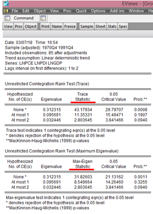
Here is the EViews result on the Johansen Cointegration test of lnpce, lnpdi and lngdp:

EViews - Johansen Cointegration Test
Source: CrucnhEconometrix

Interpreting Johansen Cointegration Test Results

1.   The EViews output releases two statistics, Trace Statistic and Max-Eigen Statistic

2.   Rejection criteria is at 0.05 level

3.   Rejection of the null hypothesis is indicated by an asterisk sign (*)

4.   Reject the null hypothesis if the probability value is less than or equal to 0.05

5.   Reject the null hypothesis if the Trace or Max-Eigen statistic is higher than the 0.05 critical value

Decision: Given the results generated, the null hypothesis of no cointegrating equation is rejected at the 5% level. Hence, it is concluded that a long-run relationship exist among the three variables.

 [Watch video on how to conduct Johansen cointegration test in EViews]

However, if the null hypothesis cannot be rejected, it evidences no cointegration and hence there is no long-run relationship among the series. This implies that, if there are shocks to the system, the model is not likely to converge in the long-run. In addition, if there is no cointegration, only the short run model should be estimated. That is, estimates only VAR do not estimate a VECM!

If there are comments or areas requiring further clarification, kindly post them below….

Panel Data Analysis (Lecture 2): How to Perform the Hausman Test in EViews

Introduction to Panel Data Models

The panel data approach pools time series data with cross-sectional data. Depending on the application, it can comprise a sample of individuals, firms, countries, or regions over a specific time period. The general structure of such a model could be expressed as follows:

Y_it = a_o + bX_it + u_it

where u_it ~ IID(0, 𝜎²) and i = 1, 2, ..., N individual-level observations, and t = 1, 2, ...,T time series observations.

In this application, it is assumed that Y_it is a continuous variable. In this model, the observations of each individual, firm or country are simply stacked over time on top of each another. This is the standard pooled model where intercepts and slope coefficients are homogeneous across all N cross-sections and through all T time periods. The application of OLS to this model ignores the temporal and spatial dimension inherent in the data and thus throws away useful information. It is important to note that the temporal dimension captures the ‘within’ variation in the data while the spatial dimension captures the ‘between’ variation in the data. The pooled OLS estimator exploits both ‘between’ and ‘within’ dimensions of the data but does not do so efficiently. Thus, in this procedure each observation is given equal weight in estimation. In addition, the unbiasedness and consistency of the estimator requires that the explanatory variables are uncorrelated with any omitted factors. The limitations of OLS in such an application prompted interest in alternative procedures. There are a number of different panel estimators but the most popular is the fixed effects (or ‘within’) estimator.

Fixed Effects or Random Effects?

The question is usually asked which econometric model an investigator should use when modelling with panel data. The different models can generate considerably different results and this has been documented in many empirical studies. In terms of a model where time effects are assumed absent for simplicity, the model to be estimated may be given by:

Y_it = a_i + bX_it + u_it

The question, therefore, is do we treat a_i as fixed or random? The following points are worth noting.

·1) The estimation of the fixed effects model is costly in terms of degrees of freedom. This is a statistical and not a computing cost. It is particularly problematic when N is large and T is small. The occurrence of large N and small T currently tends to characterize most panel data applications encountered.

·2) The a_i terms are taken to characterize (for want of a better expression) investigator ignorance. In the fixed effects model does it make sense to treat one type of investigator ignorance (a_i) as fixed but another as random (u_it)?

·3) The fixed effects formulation is viewed as one where investigators make inferences conditional on the fixed effects in the sample.

 4)The random effects formulation is viewed as one where investigators make unconditional inferences with respect to the population of all effects.

· 5) The random effects formulation treats the random effects as independent of the explanatory variables (i.e. E(a_i X_it) = 0). Violation of this assumption leads to bias and inconsistency in the b vector.

Advantage and disadvantage of the fixed effects model

The main advantage of the fixed effects model is its relative ease of estimation and the fact that it does not require independence of the fixed effects from the other included explanatory variables. The main disadvantage is that it requires estimation of N separate intercepts. This causes problems because much of the variation that exists in the data may be used up in estimating these different intercept terms. As a consequence, the estimated effects (the bs) for other explanatory variables in the regression model may be imprecisely estimated. These might represent the more important parameters of interest from the perspective of policy. As noted above the fixed effects estimator is derived using the deviations between the cross-sectional observations and the long-run average value for the cross-sectional unit. This problem is most acute, therefore, when there is little variation or movement in the characteristics over time, that is when the variables are rarely-changing or they are time-invariant. In essence, the effects of these variables are eliminated from the analysis.

Advantage and disadvantage of the random effects model

The main advantage of the random effects estimator is that it uses up fewer degrees of freedom in estimation and allows for the inclusion of time invariant covariates. The main disadvantage of the model is the assumption that the random effects are independent of the included explanatory variables. It is fairly plausible that there may be unobservable attributes not included in the regression model that are correlated with the observable characteristics. This procedure, unlike fixed effects, does not allow for the elimination of the omitted heterogeneous effects.

The Hausman Test

In determining which model is the more appropriate to use, a statistical test can be implemented. The Hausman test compares the random effects estimator to the ‘within’ estimator. If the null is rejected, this favours the ‘within’ estimator’s treatment of the omitted effects (i.e., it favours the fixed effects but only relative to the random effects). The use of the test in this case is to discriminate between a model where the omitted heterogeneity is treated as fixed and correlated with the explanatory variables, and a model where the omitted heterogeneity is treated as random and independent of the explanatory variables.

·      If the omitted effects are uncorrelated with the explanatory variables, the random effects estimator is consistent and efficient. However, the fixed effects estimator is consistent but not efficient given the estimation of a large number of additional parameters (i.e., the fixed effects).

·      If the effects are correlated with the explanatory variables, the fixed effects estimator is consistent but the random effects estimator is inconsistent. The Hausman test provides the basis for discriminating between these two models and the matrix version of the Hausman test is expressed as:

[b_RE– b_FE][V(b_FE) – V(b_RE)]^-1[b_RE – b_FE]′ ~   𝝌²_k

where k is the number of covariates (excluding the constant) in the specification. If the random effects are correlated with the explanatory variables, then there will be a statistically significant difference between the random effects and the fixed effects estimates. Thus, the null and alternative hypotheses are expressed as:

            H₀: Random effects are independent of explanatory variables

H₁: H₀ is not true.

The null hypothesis is the random effects model and if the test statistic exceeds the relevant critical value, the random effects model is rejected in favour of the fixed effects model. In finite samples the inversion of the matrix incorporating the difference in the variance-covariance matrices may be negative-definite (or negative semi-definite) thus yielding non-interpretable values for the chi-squared.

The selection of one model over the other might be dictated by the nature of the application. For example, if the cross-sectional units were countries and states, it may be plausible to assume that the omitted effects are fixed in nature and not the outcome of a random draw. However, if we are dealing with a sample of individuals or firms drawn from a population, the assumption of a random effects model has greater appeal. However, the choice of which model to choose is ultimately dictated empirically. If it does not prove possible to discriminate between the two models on the basis of the Hausman test, it may be safest to use the fixed effects model, where the consequences of a correlation between the fixed effects and the explanatory variables are less devastating than is the case with the random effects model where the consequences of failure result in inconsistent estimates. Of course, if the random effects are found to be independent of the covariates, the random effects model is the most appropriate because it provides a more efficient estimator than the fixed effects estimator.

**This tutorial is culled from my lecture note as given by Prof. Barry Reilly (Professor of Econometrics, University of Sussex, UK).

How to Perform the Hausman Test in EViews

First: Load file into EViews and create Group data (see video on how to do this)

Second: Perform fixed effects estimation: Quick >> Estimate Equation >> Panel Options >> Fixed >> OK

EViews: Equation Estimation Dialog Box
Source: CrunchEconometrix

Third: Perform random effects estimation: Quick >> Estimate Equation >> Panel Options >> Random >> OK

Fourth: Perform the Hausman test: View >> Fixed/Random Effects testing >> Correlated Random Effects – Hausman Test

Fifth: Interpret results:

Reject the null hypothesis if the prob-value is statistically significant at 5% level. It implies that the individual effects (a_i) correlate with the explanatory variables. Therefore use the fixed effect estimator to run the analysis. Otherwise, use the random effects estimator.

[Watch video tutorial on performing the Hausman test in EViews]

If you still have comments or questions regarding how to perform the Hausman test, kindly post them in the comments section below…..