Panel Data Analysis (Lecture 2): How to Perform the Hausman Test in EViews

Introduction to Panel Data Models

The panel data approach pools time series data with cross-sectional data. Depending on the application, it can comprise a sample of individuals, firms, countries, or regions over a specific time period. The general structure of such a model could be expressed as follows:

Y_it = a_o + bX_it + u_it

where u_it ~ IID(0, 𝜎²) and i = 1, 2, ..., N individual-level observations, and t = 1, 2, ...,T time series observations.

In this application, it is assumed that Y_it is a continuous variable. In this model, the observations of each individual, firm or country are simply stacked over time on top of each another. This is the standard pooled model where intercepts and slope coefficients are homogeneous across all N cross-sections and through all T time periods. The application of OLS to this model ignores the temporal and spatial dimension inherent in the data and thus throws away useful information. It is important to note that the temporal dimension captures the ‘within’ variation in the data while the spatial dimension captures the ‘between’ variation in the data. The pooled OLS estimator exploits both ‘between’ and ‘within’ dimensions of the data but does not do so efficiently. Thus, in this procedure each observation is given equal weight in estimation. In addition, the unbiasedness and consistency of the estimator requires that the explanatory variables are uncorrelated with any omitted factors. The limitations of OLS in such an application prompted interest in alternative procedures. There are a number of different panel estimators but the most popular is the fixed effects (or ‘within’) estimator.

Fixed Effects or Random Effects?

The question is usually asked which econometric model an investigator should use when modelling with panel data. The different models can generate considerably different results and this has been documented in many empirical studies. In terms of a model where time effects are assumed absent for simplicity, the model to be estimated may be given by:

Y_it = a_i + bX_it + u_it

The question, therefore, is do we treat a_i as fixed or random? The following points are worth noting.

·1) The estimation of the fixed effects model is costly in terms of degrees of freedom. This is a statistical and not a computing cost. It is particularly problematic when N is large and T is small. The occurrence of large N and small T currently tends to characterize most panel data applications encountered.

·2) The a_i terms are taken to characterize (for want of a better expression) investigator ignorance. In the fixed effects model does it make sense to treat one type of investigator ignorance (a_i) as fixed but another as random (u_it)?

·3) The fixed effects formulation is viewed as one where investigators make inferences conditional on the fixed effects in the sample.

 4)The random effects formulation is viewed as one where investigators make unconditional inferences with respect to the population of all effects.

· 5) The random effects formulation treats the random effects as independent of the explanatory variables (i.e. E(a_i X_it) = 0). Violation of this assumption leads to bias and inconsistency in the b vector.

Advantage and disadvantage of the fixed effects model

The main advantage of the fixed effects model is its relative ease of estimation and the fact that it does not require independence of the fixed effects from the other included explanatory variables. The main disadvantage is that it requires estimation of N separate intercepts. This causes problems because much of the variation that exists in the data may be used up in estimating these different intercept terms. As a consequence, the estimated effects (the bs) for other explanatory variables in the regression model may be imprecisely estimated. These might represent the more important parameters of interest from the perspective of policy. As noted above the fixed effects estimator is derived using the deviations between the cross-sectional observations and the long-run average value for the cross-sectional unit. This problem is most acute, therefore, when there is little variation or movement in the characteristics over time, that is when the variables are rarely-changing or they are time-invariant. In essence, the effects of these variables are eliminated from the analysis.

Advantage and disadvantage of the random effects model

The main advantage of the random effects estimator is that it uses up fewer degrees of freedom in estimation and allows for the inclusion of time invariant covariates. The main disadvantage of the model is the assumption that the random effects are independent of the included explanatory variables. It is fairly plausible that there may be unobservable attributes not included in the regression model that are correlated with the observable characteristics. This procedure, unlike fixed effects, does not allow for the elimination of the omitted heterogeneous effects.

The Hausman Test

In determining which model is the more appropriate to use, a statistical test can be implemented. The Hausman test compares the random effects estimator to the ‘within’ estimator. If the null is rejected, this favours the ‘within’ estimator’s treatment of the omitted effects (i.e., it favours the fixed effects but only relative to the random effects). The use of the test in this case is to discriminate between a model where the omitted heterogeneity is treated as fixed and correlated with the explanatory variables, and a model where the omitted heterogeneity is treated as random and independent of the explanatory variables.

·      If the omitted effects are uncorrelated with the explanatory variables, the random effects estimator is consistent and efficient. However, the fixed effects estimator is consistent but not efficient given the estimation of a large number of additional parameters (i.e., the fixed effects).

·      If the effects are correlated with the explanatory variables, the fixed effects estimator is consistent but the random effects estimator is inconsistent. The Hausman test provides the basis for discriminating between these two models and the matrix version of the Hausman test is expressed as:

[b_RE– b_FE][V(b_FE) – V(b_RE)]^-1[b_RE – b_FE]′ ~   𝝌²_k

where k is the number of covariates (excluding the constant) in the specification. If the random effects are correlated with the explanatory variables, then there will be a statistically significant difference between the random effects and the fixed effects estimates. Thus, the null and alternative hypotheses are expressed as:

            H₀: Random effects are independent of explanatory variables

H₁: H₀ is not true.

The null hypothesis is the random effects model and if the test statistic exceeds the relevant critical value, the random effects model is rejected in favour of the fixed effects model. In finite samples the inversion of the matrix incorporating the difference in the variance-covariance matrices may be negative-definite (or negative semi-definite) thus yielding non-interpretable values for the chi-squared.

The selection of one model over the other might be dictated by the nature of the application. For example, if the cross-sectional units were countries and states, it may be plausible to assume that the omitted effects are fixed in nature and not the outcome of a random draw. However, if we are dealing with a sample of individuals or firms drawn from a population, the assumption of a random effects model has greater appeal. However, the choice of which model to choose is ultimately dictated empirically. If it does not prove possible to discriminate between the two models on the basis of the Hausman test, it may be safest to use the fixed effects model, where the consequences of a correlation between the fixed effects and the explanatory variables are less devastating than is the case with the random effects model where the consequences of failure result in inconsistent estimates. Of course, if the random effects are found to be independent of the covariates, the random effects model is the most appropriate because it provides a more efficient estimator than the fixed effects estimator.

**This tutorial is culled from my lecture note as given by Prof. Barry Reilly (Professor of Econometrics, University of Sussex, UK).

How to Perform the Hausman Test in EViews

First: Load file into EViews and create Group data (see video on how to do this)

Second: Perform fixed effects estimation: Quick >> Estimate Equation >> Panel Options >> Fixed >> OK

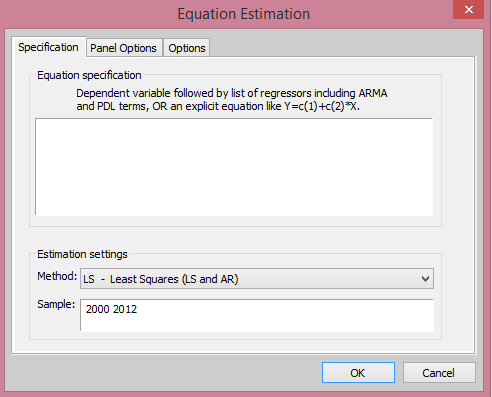
EViews: Equation Estimation Dialog Box
Source: CrunchEconometrix

Third: Perform random effects estimation: Quick >> Estimate Equation >> Panel Options >> Random >> OK

Fourth: Perform the Hausman test: View >> Fixed/Random Effects testing >> Correlated Random Effects – Hausman Test

Fifth: Interpret results:

Reject the null hypothesis if the prob-value is statistically significant at 5% level. It implies that the individual effects (a_i) correlate with the explanatory variables. Therefore use the fixed effect estimator to run the analysis. Otherwise, use the random effects estimator.

[Watch video tutorial on performing the Hausman test in EViews]

If you still have comments or questions regarding how to perform the Hausman test, kindly post them in the comments section below…..

Panel Data Analysis (Lecture 2): How to Perform the Hausman Test in Stata

 

Introduction to Panel Data Models

The panel data approach pools time series data with cross-sectional data. Depending on the application, it can comprise a sample of individuals, firms, countries, or regions over a specific time period. The general structure of such a model could be expressed as follows:

Y_it = a_o + bX_it + u_it

where u_it ~ IID(0, 𝜎²) and i = 1, 2, ..., N individual-level observations, and t = 1, 2, ...,T time series observations.

In this application, it is assumed that Y_it is a continuous variable. In this model, the observations of each individual, firm or country are simply stacked over time on top of each another. This is the standard pooled model where intercepts and slope coefficients are homogeneous across all N cross-sections and through all T time periods. The application of OLS to this model ignores the temporal and spatial dimension inherent in the data and thus throws away useful information. It is important to note that the temporal dimension captures the ‘within’ variation in the data while the spatial dimension captures the ‘between’ variation in the data. The pooled OLS estimator exploits both ‘between’ and ‘within’ dimensions of the data but does not do so efficiently. Thus, in this procedure each observation is given equal weight in estimation. In addition, the unbiasedness and consistency of the estimator requires that the explanatory variables are uncorrelated with any omitted factors. The limitations of OLS in such an application prompted interest in alternative procedures. There are a number of different panel estimators but the most popular is the fixed effects (or ‘within’) estimator.

Fixed Effects or Random Effects?

The question is usually asked which econometric model an investigator should use when modelling with panel data. The different models can generate considerably different results and this has been documented in many empirical studies. In terms of a model where time effects are assumed absent for simplicity, the model to be estimated may be given by:

Y_it = a_i + bX_it + u_it

The question, therefore, is do we treat a_i as fixed or random? The following points are worth noting.

·  The estimation of the fixed effects model is costly in terms of degrees of freedom. This is a statistical and not a computing cost. It is particularly problematic when N is large and T is small. The occurrence of large N and small T currently tends to characterize most panel data applications encountered.

·   The a_i terms are taken to characterize (for want of a better expression) investigator ignorance. In the fixed effects model does it make sense to treat one type of investigator ignorance (a_i) as fixed but another as random (u_it)?

·      The fixed effects formulation is viewed as one where investigators make inferences conditional on the fixed effects in the sample.

·  The random effects formulation is viewed as one where investigators make unconditional inferences with respect to the population of all effects.

·  The random effects formulation treats the random effects as independent of the explanatory variables (i.e. E(a_i X_it) = 0). Violation of this assumption leads to bias and inconsistency in the b vector.

Advantage and disadvantage of the fixed effects model

The main advantage of the fixed effects model is its relative ease of estimation and the fact that it does not require independence of the fixed effects from the other included explanatory variables. The main disadvantage is that it requires estimation of N separate intercepts. This causes problems because much of the variation that exists in the data may be used up in estimating these different intercept terms. As a consequence, the estimated effects (the bs) for other explanatory variables in the regression model may be imprecisely estimated. These might represent the more important parameters of interest from the perspective of policy. As noted above the fixed effects estimator is derived using the deviations between the cross-sectional observations and the long-run average value for the cross-sectional unit. This problem is most acute, therefore, when there is little variation or movement in the characteristics over time, that is when the variables are rarely-changing or they are time-invariant. In essence, the effects of these variables are eliminated from the analysis.

Advantage and disadvantage of the random effects model

The main advantage of the random effects estimator is that it uses up fewer degrees of freedom in estimation and allows for the inclusion of time invariant covariates. The main disadvantage of the model is the assumption that the random effects are independent of the included explanatory variables. It is fairly plausible that there may be unobservable attributes not included in the regression model that are correlated with the observable characteristics. This procedure, unlike fixed effects, does not allow for the elimination of the omitted heterogeneous effects.

The Hausman Test

In determining which model is the more appropriate to use, a statistical test can be implemented. The Hausman test compares the random effects estimator to the ‘within’ estimator. If the null is rejected, this favours the ‘within’ estimator’s treatment of the omitted effects (i.e., it favours the fixed effects but only relative to the random effects). The use of the test in this case is to discriminate between a model where the omitted heterogeneity is treated as fixed and correlated with the explanatory variables, and a model where the omitted heterogeneity is treated as random and independent of the explanatory variables.

·      If the omitted effects are uncorrelated with the explanatory variables, the random effects estimator is consistent and efficient. However, the fixed effects estimator is consistent but not efficient given the estimation of a large number of additional parameters (i.e., the fixed effects).

·      If the effects are correlated with the explanatory variables, the fixed effects estimator is consistent but the random effects estimator is inconsistent. The Hausman test provides the basis for discriminating between these two models and the matrix version of the Hausman test is expressed as:

[b_RE– b_FE][V(b_FE) – V(b_RE)]^-1[b_RE – b_FE]′ ~   𝝌²_k

where k is the number of covariates (excluding the constant) in the specification. If the random effects are correlated with the explanatory variables, then there will be a statistically significant difference between the random effects and the fixed effects estimates. Thus, the null and alternative hypotheses are expressed as:

H₀: Random effects are independent of explanatory variables

H₁: H₀ is not true.

The null hypothesis is the random effects model and if the test statistic exceeds the relevant critical value, the random effects model is rejected in favour of the fixed effects model. In finite samples the inversion of the matrix incorporating the difference in the variance-covariance matrices may be negative-definite (or negative semi-definite) thus yielding non-interpretable values for the chi-squared.

The selection of one model over the other might be dictated by the nature of the application. For example, if the cross-sectional units were countries and states, it may be plausible to assume that the omitted effects are fixed in nature and not the outcome of a random draw. However, if we are dealing with a sample of individuals or firms drawn from a population, the assumption of a random effects model has greater appeal. However, the choice of which model to choose is ultimately dictated empirically. If it does not prove possible to discriminate between the two models on the basis of the Hausman test, it may be safest to use the fixed effects model, where the consequences of a correlation between the fixed effects and the explanatory variables are less devastating than is the case with the random effects model where the consequences of failure result in inconsistent estimates. Of course, if the random effects are found to be independent of the covariates, the random effects model is the most appropriate because it provides a more efficient estimator than the fixed effects estimator.

**This tutorial is culled from my lecture note as given by Prof. Barry Reilly (Professor of Econometrics, University of Sussex, UK).

How to Perform the Hausman Test in Stata

First: Open a log file, load data into Stata, use a do-file (to replicate your research)

Second: Inform Stata that you are using a panel with ‘id’ the cross-sectional indicator and 'year' the time period indicator to prepare for panel data analysis.

xtset id year

Third: Create year dummies (to capture time variations in the data)

tab year, gen(yr)

Fourth: Run the fixed effects model and store the results

eststo fixed: xtreg y x₁ x₂ x₃ x₄ yr2 – yr..., fe i(c_id)

Fifth: Run the random effects model and store the results

eststo random: xtreg y x₁ x₂ x₃ x₄ yr2 – yr..., re i(c_id)

Sixth: Run the Hausman test

hausman fixed random

Seventh: Interpret results: Reject the null hypothesis if the prob-value is statistically significant at 5% level. It implies that the individual effects (a_i) correlate with the explanatory variables. Therefore use the fixed effect estimator to run the analysis. Otherwise, use the random effects estimator.

[Watch video tutorial on performing the Hausman test in Stata]

If you still have comments or questions regarding how to perform the Hausman test, kindly post them in the comments section below…..

Panel Data Analysis (Lecture 1): Sourcing Data, Theoretical Framework and Model Specification

Caution: This tutorial is only a guide and should not be adopted in its entirety. Endeavour to consult your tutor and other resource materials for proper guidance!

Introduction

The dissertation fervor is heating up with the usual twists and turns. In view of these and in response to readers’ requests, I will be starting a series of lectures on how to run time series and panel data analyses. These will be in parts and supported with short video tutorials posted to YouTube (so ensure to hook up to get the hands-on training). In order not to leave anyone out, these practical lectures will be carried out using three (3) analytical packages that is common among final-year students – Stata, EViews and Excel. Also, real country-level and longitudinal data will be used (but subject to my modifications to prevent unethical conduct from readers). Lastly, only quantitative research will be addressed.

For time series analysis, the lectures will only cover: data sourcing, model specification, lag selection, unit root testing, cointegration test, vector autoregressive model (VAR), autoregressive distributed lag model (ARDL), vector error correction mechanism (VECM), Granger causality tests, CUSUMSQ test and other post-estimation tests. While for panel data analysis, the lectures will only cover: setting up a panel data in Stata and EViews, data sourcing, model specification, Hausman test, fixed effects (FE) model, random effects (RE) model and generalised methods of moments (GMM).

So, in order to get prompt tutorials, the moment I click the “post” button, I will encourage you to subscribe for these blog posts. Use the “Follow by Email” menu on my blog https://cruncheconometrix.blogspot.com.ng, activate the link once you receive the notification in your email (check your spam box too) and you are good to go! Likewise, follow that up by subscribing to my YouTube videos for those short hands-on video clips. Click on this link CrunchEconometrix YouTube videos and subscribe!

Data Sourcing

“I can’t get data!!!”, “what’s a proxy?”, “I have data but not for all the groups”,“ how do I go about modeling my theoretical framework?”, “how do I construct my empirical model?”, “in fact, I’m confused!”…so many questions and believe me the chattering seems endless. First, I always tell students to relax! Secondly, I tell them that the moment the research area has been identified, and the topic streamlined, the next thing to do is to go on data-search. Okay, think about this: of what use is an empirical research if there is no data (or you have insufficient data to test your hypothesis)? So before, you proceed to writing chapter 1 (that is, the study background), make certain that you have the data handy.

Primary Data Sources

Regardless of the field of study or research discipline, primary data gathering requires the use of questionnaires, interviews, focus group discussions etc. It may require one of these or a combination of 2 or 3 data-gathering methods. So, if you are using primary data, ensure to get out these materials and distribute to the respondents in order to harvest responses within the shortest time frame. Getting a good number of responses is a precursor to having a quality research and unbiased results. However, these structured tutorials will not be extended to analysing primary data….my sincere apologies!

Secondary Data Sources

Since, research is not limited to those in the field of economics, it is important that researchers identify those databases hosting the relevant data required for their work. As an economist, I will indicate some databases/sources where students can go source for their data. Here are some which can be accessed (for macro and micro datasets):

IEA Coal Information

IEA CO2 Emissions from Fuel Combustion

IEA Electricity information

IEA Energy Prices and Taxes

IEA Energy Technology Research and Development Database

IEA Natural Gas Information

IEA Oil Information

IEA Renewables Information

IEA World Energy Statistics and Balances

ILO Key Indicators of the Labour Market

IMF Balance of Payment Statistics

IMF Direction of Trade Statistics

IMF Government Finance Statistics

IMF International Financial Statistics

IMF World Economic Outlook

OECD Education Statistics

OECD Globalisation

OECD International Development

OECD International Direct Investment Statistics

OECD International Migration Statistics

OECD International Trade by Commodities Statistics

OECD Main Economic Indicators

OECD Main Science and Technology Indicators

OECD National Accounts

OECD Quarterly Labour Force Statistics

OECD Services Statistics

OECD Social Expenditure Database

OECD Structural Analysis

UNIDO Industrial Demand Supply

UNIDO Industrial Statistics

World Bank Global Development Finance

World Bank World Development Indicators

World Bank Africa Development Indicators

Other sources of international data include but not limited to:

World Bank - http://data.worldbank.org/data-catalog/

International Monetary Fund - http://www.imf.org/external/data.htm#data

United Nations - http://data.un.org/

http://unstats.un.org/unsd/databases.htm

Data on aid flows complied by OECD - http://www.oecd.org/dac/stats/

NBER data sets - http://www.nber.org/data/

For information from over 256 and regions since 1960, the accessible databases are:

World Development Indicators

Global Development Finance

The African Development Indicators

Doing Business

Education Statistics

Enterprise Surveys

Gender Statistics

Health Nutrition and Population Statistics

Millennium Development Goals

Worldwide Governance Indicators

Endeavour to check out those sites that are relevant to your study.

Note: it is expected that you state your data source in your thesis/dissertation and the years of coverage say 1980 to 2016, or 1970 to 2015 etc.

What is a Panel Data?

The panel data approach pools time series data with cross-sectional data. Depending on the application, it can comprise a sample of individuals, firms, countries, or regions over a specific time period. The general structure of such a model could be expressed as follows:

Y_it = a + bX_it + u_it 

where u_it ~ IID(0, s²),i = 1,2,…,N individual-level observations, and t = 1, 2,…,T time series observations.

In this application, it is assumed that Y_it is a continuous variable. The panel data model is simply where the observations of each individual, firm or country over time are stacked on top of each another. This is the standard pooled model where intercepts and slope coefficients are homogeneous across all N cross-sections and through all T time periods. The application of ordinary least squares (OLS) to this model ignores the temporal and spatial dimension inherent in the data and thus throws away useful information. It is important to note that the temporal dimension captures the ‘within’ variation in the data while the spatial dimension captures the ‘between’ variation in the data. The pooled OLS estimator exploits both ‘between’ and ‘within’ dimensions of the data but does not do so efficiently. Thus, in this procedure each observation is given equal weight in estimation. In addition, the unbiasedness and consistency of the estimator requires that the explanatory variables are uncorrelated with any omitted factors. The limitations of OLS in such an application prompted interest in alternative procedures. There are a number of different panel estimators but the most popular is the fixed effects (or ‘within’) estimator and this will be reviewed extensively here. Lastly, the generalized methods of moments (GMM) estimator will be discussed given its relevance to dynamic panel modelling.

Some Advantages of Panel Data Analysis

Panel data analysis has quite a number of distinct advantages over time series and cross-section analysis:

·   Panel (or longitudinal) data allows a researcher to analyse a number of important economic questions not readily answerable by either a cross-section or a time-series dataset alone.

·  The availability of panel data increases the number of data points available and reduces collinearity among the explanatory variables thus improving the efficiency of the econometric estimates.

·  Panel data captures the heterogeneity that is related to the individuals, firms, states, countries etc. over time.

· By combining time series of cross-sectional observations, panel data gives “more informative data, more variability, less collinearity among variables, more degrees of freedom and more efficiency”.

·    Dynamic effects cannot be estimated using cross-sectional data. Even time series data are imprecise in this regard as there is generally limited change or variation in the data to identify such effects. For instance, in estimating a distributed lag model using only time series data, multicollinearity lowers the precision of the estimates. Hence, panel data models can provide greater variation in the explanatory variable for a given year thus reducing the degree of multicollinearity and improving the precision of the estimates. This clearly renders panel data better suited to the study of dynamic change However, it should be emphasised that the estimation procedures required for dynamic models which include a lagged dependent variable are not straightforward and this issue is the subject of discussion in later sections.

· Panel data models can take into account a greater degree of the heterogeneity that characterize individuals, states, and firms over time.

(Detailed discussion on the rudiments of panel data analysis will be done in the next tutorial).

(Here is the link to video clip on converting wide-format data to long-format in Stata).

Model Framework and Specification

This section focusses on the theoretical framework and model specification. I will also touch on description of variables in a model, the a priori expectations and finally, the method of analysis (or the estimation technique(s) to be used in testing the research hypothesis).

Theoretical Framework

Before you specify the empirical model, you must first state the theoretical model. That is, let your readers know where your empirical model is linked to. The theoretical model is that model supporting the theory you are using to undertake your research because no research can be done in isolation without an underlying theory. For instance, if my study is on the effect of exchange rate on output for 30 countries from 2000 to 2016 (that is, 17years), then I must look for a suitable theory which I can adapt to my research. Hence, I may decide to use the “monetary model of exchange rate” which is one of the earliest models used to determine the exchange rate. It is used as a measure to study the other approaches that are used in determining exchange rate. The monetary model approach assumes a simple demand for money curve, the purchasing power parity or the law of one price and a vertical aggregate supply curve.

The theoretical framework can be built as follows: (remember that this is just an example, and should not to be copied literarily!)

From the absolute purchasing power parity (P = EP*), the exchange rate is obtained by dividing the price of the domestic currency by the foreign price for that domestic currency. That is: E^ppp = P/P*. The demand for money assumption: since real money balance depends on real income, demand for money is given as M_d = kPY, where k is constant and Y is the real income level. Hence, in equilibrium, money demand (M_d) equals money supply (M_s) and at the point of intersection of the aggregate demand and the aggregate supply curve:

kPY=M_s

P = M_s/kY

EP* = P = M_s/kY

and E = M_s/P*kY

From the stated framework, it is theorised that if the money supply within an economy increases, it will result in appreciation of the domestic currency. Hence, if it is generalised for the 30 countries in the data, the same assumption must be made, ceteris paribus. Likewise, foreign price level and the output level are inversely related to the exchange rate. If fixed money supply rises in the domestic economy, since prices are held constant, excess money supply leads to higher demand for goods and services within the economy.

Model Specification

So, having stated the theoretical framework, I can now go ahead to modify it to suit my research and form there formulate my empirical model. For instance, in using a Cobb-Douglas production from the neo-classical growth mode, I will attempt to explain output growth in the context of capital accumulation, labour and productivity, usually referred to as technological progress. The Cobb- Douglas production model is implicitly stated as:

Y = f(AL_βK_α)                                                                                    [1]

where, Y is output; K is capital stock; L is labour and A is productivity of labour which grows at an exogenous rate. As a result of constant returns to scale, if all inputs are increased by the same amount, then there would be an increase in output. The production function,

Y = K^αL^1-α                                                                                         [2]

where (1 - a = b) is mainly used by economists and researchers due to the following reasons: firstly, there is a constant return to scale and secondly, the two exponents α and (1 - a), sum up to one.

Next, is to tie up the empirical model to the theoretical framework. That is given the relationship between exchange rate and output, the model is implicitly specified as:

Y_it = f (Exchrate_it, X_1it, X_2it, …, X_nit)                                          [3]

where Y_it = output (the dependent variable, state the measurement either gross output, or % of GDP, or growth rate etc.)

Exchrate_it = real exchange rate (main explanatory variable)

X_1it, X_2it, …, X_nit = control variables (state their individual measurements either gross output, or % of GDP, or growth rate etc.)

On the basis of the theoretical framework and using the Cobb-Douglas production, the explicit model is stated as:

Y_it = β₀ + β₁Exchrate_it + β₂X_1it + β₃X_2it + … + β_nX_nit + u_it        [4]

where, u_t = white noise error term

 A Priori Expectations

Always know that the expected a priori is directly related to what theory says. It is from that you know what signs of the coefficients are expected from the main regressor and other covariates. For instance, from the theory, it is expected that currency depreciation will have a positive impact on domestic output, hence, a negative sign of the coefficient is expected. That is:

β₁ < 0

Therefore, the expected signs of the control variables must be in line with their respective theories which must be related to your study.

Estimation Technique

At this point, the researcher may not know the exact technique or estimator to adopt between the fixed-effects within-group (fixed effects model) or the random effects estimator. The choice between these two is subject to the outcome of the Hausman test.

That is, to determine which model is the more appropriate to adopt, a statistical test is implemented. The Hausman test compares the random effects estimator to the ‘within’ estimator. The null hypothesis of the test is that the composite error term is not correlated with the explanatory variables in the model. If the null is rejected, then the fixed effects estimator is applicable (i.e., it favours the fixed effects but only relative to the random effects). The use of the test in this case is to discriminate between a model where the omitted heterogeneity is treated as fixed and correlated with the explanatory variables, and a model where the omitted heterogeneity is treated as random and independent of the explanatory variables.

Variables, Measurement and Description

Lastly, tabulate your variables detailing their names, short description, measurement and sources.

Here’s an example:

Table xxx: Variables Description and Measurement

Variables	Short Definition	Measurement	Source
Output			World Bank (2016)
Real exchange rate			World Bank (2016)

If you have any comments or question in relation to what have been discussed in this post, do not hesitate to post them in the comment section below….

Source: Researcher’s compilation (always put this at the bottom of the Table)

Conclusion

I have taken you through the steps required on how to source for your data, in addition to a brief on panel data analysis and its relevance over time series and cross-sectional data. I also briefly explained how to formulate a theoretical framework, adapting the framework to align with the research, how to construct the empirical model, stating the expected a priori, having an idea about the estimation technique with a brief on the Hausman test, tabulating your data showing the brief description of your variables, their measurements and data sources.

From next lecture, I will begin analysing the data using both Stata and EViews analytical packages. So, endeavour to follow these tutorials by getting the most of it to ease the dissertation pressure. Make sure you follow me on the next lecture series which is: Panel Data Analysis (Lecture 2): Setting up panel data model and the Hausman Test.

If you have any comments or question in relation to what have been discussed, do not hesitate to post them in the comment section below….